My AWS Fargate Startup Times are Slow

Posted on November 26, 2025 by Dror Speiser

I’m giving a talk today at the AWS User Group Ljubljana about my attempt at making AWS Fargate container startup times shorter by playing around with layer sizes for a given image.

I failed at my goal, the startup times on Fargate are still the same for me, but my idea works great for AWS ECS over EC2 or any other docker runtime that isn’t Fargate, so yey.

I might turn the presentation into a post later, but until then the slides are available at here.

Algebraic Locality-Sensitive Hashing

Posted on August 1, 2024 by Dror Speiser

This piece presents a new family of hash functions from sequences of letters to vectors of numbers which are both locality-sensitive and algebraic. The hash functions can also be used with other inputs such as images, time series, multi-dimensional arrays, and even arrays with varying dimensions. We’ll go over examples and see some animations.

Intro

Sometimes we are handed a collection of objects and we need to find which are similar and which aren’t. For example we might be looking at articles in English on Wikipedia, and we want to find pairs that are very similar. Or maybe we’re looking at DNA sequences and we’re interested in understanding similarity between species. Further afield, we might have a large collection of image files and we want to check if we have one that is similar to an image that someone sent us. Maybe it’s stock price series over 10 ten years instead of images. In all these cases we aren’t looking for exact matches, but rather similar objects, where we have some notion of similarity.

Levenshtein distance

If our collection of objects is that of strings, meaning sequences of letters, then there are a few such notions of similarity that are popular, the most prominent being Levenshtein distance. The Levenshtein distance between two strings is the number of operations needed to go from one to the other, where the allowed operations are adding a letter, deleting a letter, and modifying a letter. For example, the Levenshtein distance between “kitten” and “sitting” is 3, and this example can be found on the Wikipedia page for Levenshtein distance.

The Levenshtein distance is very useful when quantifying the distance between two strings. Unfortunately, it is also pretty time consuming to compute, especially if the strings are long. Computing the Levenshtein distances of all pairs from a large collection of strings is time consuming and often infeasible.

Locality-sensitive hashes and MinHash

Instead of computing the distance between all pairs of strings from a collection, we can employ the idea of first hashing, meaning mapping, all the strings with a function that is locality-sensitive. This means that the hashes of a pair of similar strings are also similar, and the hashes of unsimilar strings are likely to be unsimilar. If we have such a hash function, then we can first apply it to all strings in our collection, and then go over only those pairs of strings whose hash values are already similar. This idea can cut down are search space considerably, turning intractable problems into tractable ones.

The most famous locality-sensitive hash function is MinHash. The actual definition is technical, and I want to keep the technical parts of this piece to the new family of hash functions, so you can read more on its great Wikipedia page.

I do want to note one thing about MinHash: it is commutative, meaning order doesn’t matter. For example, if we’re using MinHash by looking at words in strings, then the hash of the sentence “don’t give up, you matter” is the same as the hash of the sentence “you don’t matter, give up”.

New locality-sensitive hash functions

Letter counting

Before delving into interesting new locality-sensitive hash function, let’s look at a subset of the family that is old and known – letter counting.

Given a large collection of strings, we can count how many times each string contains the letter “a”. We can then go over pairs that have a similar number of a’s and compute their Levenshtein distance. This idea can cut down out search space by some factor. We can also count the number of b’s in each string, and then use the two counts together to cut down the number of pairs we go over. We can do this for a few letters, though generally speaking we can’t use too many since it’s not trivial or clear how to enumerate only those pairs of strings that have a similar number of a’s, b’s, etc. We can use data structures such as k-d trees or R-trees.

Two things to note about this family of hash functions: first, it satisfies the first part of the (loose) definition of locality-sensitive hash functions appearing above, meaning similar strings will have similar counts of a’s, b’s, etc. On the other hand, it’s not clear that letter counting satisfies the other half of the definition, meaning unsimilar strings might not be that unlikely to have similar letter counts. This comes down to the statistical fact that letter frequencies in a given language’s texts might not be all that random.

Second, these hash functions are also commutative, meaning order doesn’t matter. In this case, it’s order of letters that doesn’t matter, so even the two words “admirer” and “married” have the same hash values.

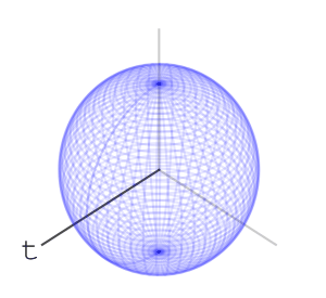
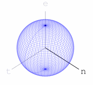
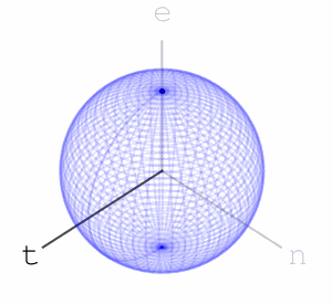
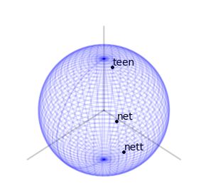
$SO(3)$ – Rotations of a ball

We will now introduce the first new locality-sensitive hash function through an example.

Let’s take three letters: “n”, “e”, “t”. Also, let’s take a sphere, a ball in 3 dimensions. Our three dimensions have 3 axes. We’ll associate the letter “n” with rotating the ball along one of the axes, exactly 35 degree:

We’ll associate the letters “e” and “t” to rotating along the other two axes, like so:

We’ll mark a point at the top of the sphere, and apply the word net. What do I mean by apply? We’ll rotate the ball first using the rotation associated with “n”, then with “e”, then with “t”, like so:

Using this idea of assigning a sequence of rotations to letters we get a function from words with these letters to points on the sphere – we apply the rotations to the marked point at the top of the sphere and the word’s hash value is where we end up.

Let’s look at two other words’ sequence of rotations applied to the marked point at the top of the sphere. Here is “nett”:

and here is “teen”:

Here are the final positions of moving the marked point using the sequences of rotations associated with the three words:

We see that “net” and “nett” move the marked point to points that are slightly closer than where “teen” moves it to, matching our intuition on the similarity of these words. We can assign a rotation to each letter of the alphabet. We can go further and assign rotations to all ascii letters, or utf8 letters. Once we’ve done that, we have a rotation associated to every word, sentence, or string in general: to apply a string’s rotation to a point we first apply the rotation of its first letter, then its second letter, and so on.

Some notes: first, general rotations of a ball, meaning elements of $SO(3)$ , are not commutative – applying one rotation and then another is generally not the same as applying them in the reverse order. If we choose somewhat random rotations for each letter in our alphabet, then our hash function does not have the commutativity property that MinHash and letter counting do. The order of letters, words, etc. matters. This could be desired, or not, and depends on the use case.

Second, similarly to MinHash, for each choice of rotations to letters we get a new hash function, and we can combine multiple such choices in order to create a new hash function. In contrast to MinHash, the computational complexity grows linearly with the number of such choices, but this is a bit too technical for this piece.

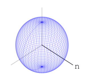
Third, we can show that similar strings move a fixed point to similar positions. What follows is the most technical part of this piece: the maximum distance a rotation $g$ can move a point is the maximal eigenvalue of $g-I$ . If we choose all our elements of $SO(3)$ so that this maximum eigenvalue is $\theta$ , for some small number $\theta$ , then applying two strings $x,y$ with Levenshtein distance $n$ to a given fixed point can only result in a Euclidean distance not greater than $2n\theta$ – each letter operation counts at most as changing two basic rotations.

Fourth, fixing a marked point and a small $\theta$ as above, experiments with Wikipedia articles hint that strings of length at least $O(1/\theta^2)$ end in a uniform-like distribution on the sphere. I can’t prove that this is indeed the case, and I’ve asked a simpler question on math.stackexchange, with no answers so far.

Fifth, if we actually use this method at the level of letters of an alphabet as the example above did, then we have a hashing method that is somewhat robust to typos, or in a biology context, to genetic mutations.

Finally, the choice of $SO(3)$ for the first example was for its ability to be easily visualized. We can use higher rotation groups – $SO(n)$ – or any algebraic group. A nice property that the special orthogonal groups have is compactness. This means the numbers in our calculations can’t go crazy, and we should expect numerical stability. I also like that they’re connected. Another family of compact connected real algebraic groups is that of special unitary groups. Which is better practically is a question of performance of representation and multiplication of elements, and I don’t know the answer right now.

Hashing other things

DNA and RNA

These can thought of strings in specific alphabets, and the above applies verbatim.

$\mathbb{R}^n$ – Fixed length vectors

Given a fixed length $n$ , we can choose $n$ elements $g_1,...,g_n$ in a connected compact real algebraic group $G$ (such as $SO(3)$ ), such that the maximal eigenvalue of $g-I$ for each element $g$ is $\theta$ , for some small $\theta$ . Fixing some point $v$ in a space on which $G$ acts (such as a point on the unit sphere), we now have the following hash function on vectors of length $n$ :

$(x_1,...,x_n)\mapsto g_1^{x_1} ... g_n^{x_n}v.$

This will satisfy the property that similar vectors map to similar points. This can be proved using the same reasoning as that given above for rotations associated with letters.

We can use such a map to compress fixed length sequences. For example, there’s a lot of talk these days about Large Language Models (LLMs), and how they give rise to embedding vectors for texts. These can have high dimension, which can be brought down to, say, dimension 9 by using the above with a group like $SO(3)\times SO(3)\times SO(3)$ (each factor contributing 3 degrees of freedom).

Images of varying dimensions

If we a have collection of images of equal dimensions, then we can choose an ordering of the pixels of these images and use the previous section’s mapping. If the images in our collections have different dimensions, then we need to look for something else.

One idea goes as follows. Pick two non-commuting elements $g,h\in G$ , for a connected real compact algebraic group $G$ , such that the maximal eigenvalues of $g-I$ and $h-I$ are small. Enumerate the values of the pixels of each image as $v_{11}, v_{12}, ..., v_{ij}, ..., v_{nm}$ (where we assume all images are gray-scale, though the following can also be done with more colors). We then have the following mapping:

$(v_{ij}) \mapsto \prod_{i=1}^n\prod_{j=1}^m\big( g^{v_{ij}}h \big).$

This mapping satisfies a type of distance-similarity property.

Time series

The same idea works verbatim for time series, where we can interpret the element $h$ in the above formula as representing the passage of time. This mapping can, for example, be used to find pairs of stocks whose series of values are similar.

General monoid

We’ve been talking about algebraic groups, but we don’t really need inverses for everything that’s been said so far, we just need the ability to multiply elements. If instead of a connected real compact algebraic group we take the monoid $(\mathbb{R}\cup{\infty},\text{min})$ and some random mapping from a given collection to $\mathbb{R}$ , then we recover MinHash. Yey!

Optimization and LLMs

In contrast to MinHash, using algebraic groups lends itself to optimization. If we have some property we want our mapping to satisfy, we can look for choices of embeddings that satisfy this property by using standard optimization algorithms.

For example, say we are interested in DNA sequences, and we want to choose four elements $g_c, g_g, g_a, g_t\in SO(3)$ , one for each nucleobase, such that the embeddings of some sample of DNA sequences is relatively uniform on the sphere. We can create a loss function that measures the uniformness of these embeddings. This loss function is then a differentiable function in the coordinates of our four elements (given a choice of representation of $SO(3)$ ), and we can minimize this loss function with standard algorithms such as SGD or Adam.

We note that using a compact group like $SO(3)$ comes in handy for this task since we can run backwards propagation with constant memory, meaning not depending on the sequences’ lengths.

Another potential application of the functions introduced in this piece is predicting tokens in a language model. Continuing our DNA example from above, we can take our loss function to be that of measuring the distance between an embedding of a subsequence of DNA and the embedding of its next nucleobase. Optimizing this loss function might give an interesting “language model” for DNA, though I haven’t done any experiments with this yet.

Conclusion

This piece has introduced a family of algebraic locality-sensitive hashing functions, that as far as the author is aware, is new. These functions can be interesting for a wide variety of contexts, such as hashing strings, images, time series, and general multi-dimensional arrays of fixed or varying dimensions. In contrast to MinHash, the functions are algebraic and differentiable, so optimization can be applied to their choice, and they should be performant on modern hardware such as GPUs.

MLE for Linear Standard Variation in Python

Posted on October 24, 2021 by Dror Speiser

The Setting

At work we’ve been looking at the variance of differences between sale prices of neighboring houses, and its dependence on the distance in space and time of the sales.

Searching for about a minute on the web, I didn’t see an implementation of a solution to the following problem:

The Problem

Given the model
$\varepsilon_i \sim \mathcal{N}(0, \langle x_i, a\rangle^2),$
and samples $(x_i, \varepsilon_i)_{i=1}^n$ , what is the maximum likelihood estimation for the vector $a$ ?

The Log-Likelihood

Using Gauss’s formula:
$\begin{aligned} \log{p(\varepsilon | a,x)} &= \log{\left( \prod_{i=1}^n \frac{1}{\sqrt{2\pi}\langle x_i, a\rangle} \exp\left(-\frac{1}{2}\frac{\varepsilon_i^2}{\langle x_i, a\rangle^2}\right) \right)} \\ &= \sum_{i=1}^n \left(-\log{\langle x_i, a\rangle - \frac{1}{2}\frac{\varepsilon_i^2}{\langle x_i, a\rangle^2}} \right) - \frac{n}{2}\log{2\pi} \end{aligned}$

The Jacobian

We’re going to use BFGS to maximize the log-likelihood, so we’ll also need the Jacobian. Differentiating the above:
$\begin{aligned} \frac{\partial\log{p(\varepsilon | a,x)}}{\partial a_j} &= \sum_{i=1}^n \left(\frac{x_{ij}}{\langle x_i, a\rangle} - \frac{\varepsilon_i^2x_{ij}}{\langle x_i, a\rangle^3} \right) \end{aligned}$

The Code

From here it’s just writing correct numpy broadcasting code and calling to scipy’s minimize. We also tack on numba.

from numba import njit
import numpy as np
import scipy.optimize

@njit
def linear_std_f_jac(a, x, e2):
    """
    Compute the minus log-likelihood of $e^2$ given the model $e~N(0, <x,a>^2)$
    (up to a fixed additive constant) and its Jacobian with respect to `a`.
    """
    dots = 1/np.dot(x, a)
    e2dots2 = e2 * dots**2
    f = np.sum(e2dots2 / 2 - np.log(dots))
    j = np.sum(x * (dots - e2dots2 * dots).reshape(-1, 1), axis=0)
    return f, j

def mle_linear_std(x, *, e=None, e2=None, a0=None, bounds=None, **kwargs):
    """
    Find the MLE for `a` given the model $e~N(0, <x,a>^2)$
    
    If you pass `e2`, the squared errors, then they won't be recomputed.
    If you don't pass `e2`, then you must pass `e`.
    
    `a0`, `bounds` and `kwargs` are passed to `scipy.optimize.minimize`.
    """
    x = np.asanyarray(x)
    assert x.ndim == 2
    n, l = x.shape
    if a0 is None:
        a0 = np.ones(l)
    else:
        a0 = np.asanyarray(a0)
    if e2 is None:
        assert e is not None
        e = np.asanyarray(e)
        assert e.ndim == 1
        e2 = e**2
    else:
        e2 = np.asanyarray(e2)
        assert e2.ndim == 1
    if bounds is None:
        bounds=[(0, None)] * l
    return scipy.optimize.minimize(
        linear_std_f_jac, a0,
        args=(x, e2), jac=True, bounds=bounds, **kwargs
    )

The Example

n = 10_000_000
l = 5

random = np.random.RandomState(1729)
x = np.c_[np.ones(n), np.abs(random.randn(n, l - 1))]
a = np.abs(random.randn(l))
e = np.dot(x, a)

import time
t1 = time.time()
res = mle_linear_std(x, e2=e**2)
t2 = time.time()

print("time:", t2 - t1)
print("correct:", a, "\n")
print(res)

Which outputs:

time: 7.45331597328186
correct: [1.70512861 0.28985998 1.05376116 1.58281698 1.39634357] 

      fun: 21011319.054358717
 hess_inv: <5x5 LbfgsInvHessProduct with dtype=float64>
      jac: array([ 5.7129652 ,  2.83110926,  4.06507689, 10.56198964, -2.42801207])
  message: 'CONVERGENCE: REL_REDUCTION_OF_F_<=_FACTR*EPSMCH'
     nfev: 13
      nit: 12
     njev: 13
   status: 0
  success: True
        x: array([1.70513432, 0.28985536, 1.0537623 , 1.5828478 , 1.39631855])

Looks ok.

A New Recipe for Idempotent Cloud Deployments

Posted on September 15, 2021 by Dror Speiser

** This post describes an idea that materialized after many many talks with Nathan and Hillel.

I’ve seen many deployment workflows and scripts, many of which use GitHub actions or equivalents, use Docker for build stages, and use terraform/cloudformation/scripts for deployment.

Once kinks are sorted out, these work really well.

The Infrastructure as Code movement is thriving, DevOps is better, and we’re happier.

Except, every time someone (usually me) pushes a weird enough merge commit on my github repo, the action to build and deploy my lambdas is triggered, the docker build is just a tiny bit different this time, and everything breaks.

Docker is not really reproducible

Unless you’re distroless and in control of everything (like Nathan is), you already know what I’m saying.

Usually it’s apt get that kills reproducibility, but it’s hardly the only danger.

Maybe always use the same machine?

One way to solve reproducibility is to always use the same machine on which you’ve done the docker builds that get deployed.

Docker will use cached layers on following builds, so the build artifacts will be the same.

But you want to use GitHub actions – so it’s always a new environment.

Replacing Reproducibility with Idempotency

I have come to terms with the fact that I cannot reproduce builds.

Not with the current technology stack I’m familiar with(*).

Instead, I’ll settle for not building a second time whatever I have already built, and not deploying a second time whatever I have already deployed.

The action of build and deploy needs to be idempotent.

Sometimes GitHub actions are presented as idempotent, in that you can set that only changes to parts of your code trigger a workflow.

But since the trigger is based on the commit tree – and not the code itself – the workflow can still trigger even if the code didn’t change.

Moreover, if a deployment is triggered for one artifact, usually this cascades into a build and deploy of all artifacts, even if the others didn’t change.

(*) There’s a package manager called Nix, and an OS called NixOS, that maybe completely solve reproducible idempotent builds and deployments, but I haven’t understood them yet.

The new recipe

I’ll present the solution I’ve started using, with the concrete choices I made, though there’s a clear general principle that can be extracted and translated into other environments.

1. Put build stages in a DVC DAG

What is DVC?

DVC is short for Data Version Control, and it is a python package for keeping track of data, machine learning experiments, and models.

Putting aside the original intent of DVC, it is perfect for idempotent builds:

You define build stages
Each stage spells out explicitly its dependencies – all the code it uses
Each stage writes explicitly its outputs – built artifacts
On rerunning, only changed stages are rerun – idempotency.

Note, though DVC is a python package, none of your code needs to be in python, and nothing in my recipe uses python. DVC is just a neat tool for pipeline and remote storage management.

Wait, why not `make`?

Yes, you can define DAGs of builds using make, and in fact this is very common.

But:

Running make a second time is idempotent only if you’re on the same machine, which you’re not, since you’re on GitHub actions.
The artifacts are not automatically stored anywhere.

What does DVC look like?

Here is a dvc.yaml file defining a single build stage:

stages:
  myapp:
    deps:
      - myapp/
      - buildmyapp.sh
    cmd: ./buildmyapp.sh
    outs:
      - "artifacts/myapp.zip"

In DVC terminology, this is a pipeline with a single stage, that depends on everything in the myapp directory, and also on the script to build the app

The stage also declares a single output, a zip file that will go in the artifacts directory.

2. Define a DVC remote

Similar to a git remote, you tell DVC where you want data files pushed to.

Generalizing the original intent of the authors of DVC, instead of pushing raw data of some kind, or some machine learning model, we will push the built zip file that is our application.

Personally, I defined my remote to be on S3.

We’ll soon talk about when to actually push the artifacts to the remote.

3. Put the deployment as a stage

To make deployment contingent on the code actually changing, all we have to do is use the DAG we have, in this case dvc.yaml.

Updating the dvc.yaml pipeline file above, it looks like this:

stages:
  myapp:
    deps:
      - myapp/
      - buildmyapp.sh
    cmd: ./buildmyapp.sh
    outs:
      - "artifacts/myapp.zip"
  deploy:
    deps:
      - artifacts/
      - deploy.sh
    cmd: ./deploy.sh

The deploy stage depends on the artifacts directory, so any time it is modified by the first stage the deploy stage will also run.

But the deploy stage can also run if only the deploy script is changed.

This is where we already can see some idempotency: if we don’t change myapp’s code, the artifact won’t change, and so its deployment won’t be affected. Even if GitHub decided to run the workflow that runs DVC.

4. The GitHub Workflow

The GitHub workflow needs to run these commands:

dvc pull \
 && dvc repro \
 && dvc push \
 && git add dvc.lock \
 && git commit -m "updated dvc.lock" \
 && git push

Of course the environment in which commands run needs to have DVC installed, as well as credentials to push to the dvc and git remotes.

dvc pull

This pulls the previously built artifacts from the DVC remote, in my case from S3.

If we changed the deploy script, but not myapp, we still need the myapp zip artifact for the deploy script to work correctly.

Since we’re pulling exactly the zip file that was deployed last, we know for certain that we aren’t changing myapp.

dvc repro

This runs the stages in the pipeline defined in dvc.yaml.

dvc push

This pushes the created artifacts to the DVC remote.

The point here is that on following builds, even if they are on different machines, we’ll still get the last built artifact from dvc pull.

This combination of dvc push and dvc pull is one of the key differences from using make.

git add+commit+push

If any of our code changed, whether it’s the myapp code, the deployment script, or both, the hashes have changed.

Hashes of pipeline dependencies are stored in a file called dvc.lock.

We push the changes to origin.

Is it ok to push from a workflow action? Won’t we get an infinite loop?

This is where idempotency is critical.

The push of dvc.lock will indeed trigger another run of the workflow.

But this time, since the code hasn’t changed since the last run, all hashes will be the same, and DVC won’t run any of the pipeline stages.

This means there won’t be anything to git push, and we won’t get a third run of the workflow.

Versioning

Questions of identity go back thousands of years.

If we change one line of code, then another, and then another, until all code has been refactored, is it still the same code?

We’ll go with no.

Code is exactly the same only if it really is exactly the same.

Assuming our hash function has few collisions, we’ll also allow for the hash of code to identify it.

Given this, in order to know the version of a deployed artifact, we just need to know its hash.

Version in Logs

The most common type of versioning requirement is that the version be printed in logs of systems running the artifact.

In my own current projects the artifacts are zip files that are deployed to AWS lambda, and these zips contain python packages.

Here is the top of my lambda function:

def lambda_handler(event, context):
    print(f"CODE_ZIP_HASH='{os.environ.get('CODE_ZIP_HASH', 'n/a')}'")

This prints (to cloudwatch) the environment variable CODE_ZIP_HASH.

I populate this variable through the definition of the lambda in the deployment script.

Specifically, my deployment script uses AWS CDK, also in python, and the relevant lines are these:

    code_zip_hash = hashlib.md5(open(zip_path, 'rb').read()).hexdigest()

    func = aws_lambda.Function(
        stack,
        "myapp",
        runtime=aws_lambda.Runtime.PYTHON_3_8,
        code=_lambda.Code.from_asset(zip_path),
        handler='lambda_function.lambda_handler',
        description="Best app ever!",
        timeout=timeout,
        environment={'CODE_ZIP_HASH': code_zip_hash}
    )

There’s an additional layer of awesomeness here: DVC also uses md5 as its hashing algorithm.

Say the md5 hash of an artifact at some point was “b0d7…”, and we see it in some log.

Even if the repo has since moved on, we can look for all commits whose dvc.lock file has this hash “b0d7…”.

Though getting the commits is helpful, remember that builds aren’t reproducible, so if we want the actual artifact corresponding to “b0d7…” we need something else.

This is where DVC’s storage model comes in to play: it stores files exactly by their hash. In fact, it’s pretty much the same way git stores blobs.

So getting this old artifact is as simple as downloading /path/to/remote/b0/d7...

What about logging the commit itself?

Of course you can do it.

You can inject the current git commit into the artifact build stage.

Since git commits aren’t unique identifiers of artifacts, I chose not to do this in my own project.

Version in Deployment

Having the version printed in logs allows us to look back at what has already run.

But what if I want to know what will run if I trigger my lambda right now?

In my project, I wanted my lambda to have its unique identifier right in its description, so just by looking in AWS Console I can know what will run next.

All I had to do is update my lambda definition above to this:

    code_zip_hash = hashlib.md5(open(zip_path, 'rb').read()).hexdigest()

    func = aws_lambda.Function(
        stack,
        "myapp",
        runtime=aws_lambda.Runtime.PYTHON_3_8,
        code=_lambda.Code.from_asset(zip_path),
        handler='lambda_function.lambda_handler',
        description=f'Best app ever! [CODE_ZIP_HASH={code_zip_hash}]',  # <-- modified line
        timeout=timeout,
        environment={'CODE_ZIP_HASH': code_zip_hash}
    )

Recap

In order to have idempotent artifact builds and cloud deployments:

Put builds and deployment as stages in a DVC pipeline.
Define all the dependencies and outputs correctly.
Use a DVC remote such as S3.
Use: dvc pull && dvc repro && dvc push && git add && git commit && git push.
It’s also easy to add identifiers and commit hashes to logs and descriptions.

The benefits are:

Changing one artifact’s code does not force rebuilding other artifacts, even if you’re building on a new VM every time.
Changing only the deployment script won’t build any artifacts at all.
You have an artifact repository that just works.
Your git history contains the hashes of all built artifacts.
You can look up any artifact using its hash.

Alternatives

The usage of DVC in the recipe is pretty basic, and you could write the infrastructure yourself instead.

It’s mostly hashing things, saving to files, checking files, and hashing some more.

Nathan pointed me to git-annex, a tool that also saves files remotely in a git-like structure, referencing files by their hashes. You can replace that part of my recipe with git-annex.

There are also other pipeline tools out there, most familiar are AirFlow, Luigi, and Prefect.

These don’t understand caching, so I’m not sure how to replace DVC’s pipeline with theirs.

There is one more pipeline tool called Dagster, which has an experimental caching option. This can indeed replace DVC’s pipeline in the recipe.

Finally, Nix should get one more mention.

Nix is supposed to solve all reproducibility and idempotency problems by saving everything by hash. Really everything. From the libraries you use, to glibc itself. I’m still looking into this.

Gotchas of deploying to ECR from github actions

Posted on June 4, 2021 by Dror Speiser

Today I got my team’s github repo at work to automatically build a docker image for day-to-day research, and push it to AWS ECR, using a github action.

It took me a couple of hours, and I want to share the things that took the longest. All of the information exists elsewhere, and in great multiplicity, but the short list of what goes wrong might help you cut two hours.

on: manual dispatch

Before making relevant pushes trigger the build, I decided on using manual dispatch.

It then took me over 15 minutes to perform the first build.

Why? Because I missed the fine print that says that the button to run a manual dispatch action only shows if the workflow is in the default branch!

Sure, it’s not really fine print, it’s just normal print. But I still missed it and wasted time looking through issues to find a solution. So:

Tip 1. Use manual dispatch at the beginning for testing – but remember to use the default branch

Once I got the action actually running, I ran into the next set of problems.

Permissions: Roles & Policies

You have to do ECR login. This is written everywhere.

You also have to create a role and give it permissions for certain actions in a policy. This is also written enough times, including on the github page of Amazon’s ecr-login action.

But it still took me a long time to understand that I should have two (!) Sids – one for getting a token, and one for everything needed for pushing the ECR image.

The major reason it took me a long time is that I kept experimenting with policies, with every time my docker image being built, and only after 7 minutes was the ECR push rejected. Thus:

Tip 2. Experiment with policies using a one-line Dockerfile until you have it working

Getting the policy working has (most likely) nothing to do with the content of your dockerfile, so you can separate the work on them.

And then there’s:

Tip 3. You need two Sids in the policy. Something like this:

{
    "Version": "2012-10-17",
    "Statement": [
      {
        "Sid": "GetAuthorizationToken",
        "Effect": "Allow",
        "Action": [
            "ecr:GetAuthorizationToken"
        ],
        "Resource": [
            "*"
        ]
      },
      {
         "Sid": "AllowPush",
         "Effect": "Allow",
         "Action": [
            "ecr:GetDownloadUrlForLayer",
            "ecr:BatchGetImage",
            "ecr:BatchCheckLayerAvailability",
            "ecr:PutImage",
            "ecr:InitiateLayerUpload",
            "ecr:UploadLayerPart",
            "ecr:CompleteLayerUpload"
         ],
         "Resource": "arn:aws:ecr:us-east-2:<<account-id>>:repository/<<repository name>>/*"
      }
    ]
  }

Take a close look at the resources allowed. These took me a while to figure out.

First:

Tip 4. You (probably) should have an asterisk in the GetAuthorizarionToken resource

I’m not an expert on this, so maybe there is a more precise resource to put that is more secure. But the error the github runner kept giving me was that I need access to “*”.

Second, the actions relevant to ECR can and should do with a more precise resource path.

But! If you’re pushing multiple images, as I am, into repositories with the same prefix, then:

Tip 5. Make sure the resource has an asterisk if it needs one

That’s it, these were the five points that took me the most time to figure out.

The whole process still took only about 2 hours, and I’m happy with the result.

Using the State Pattern to Reduce Cyclomatic Complexity

Posted on September 30, 2018 by Dror Speiser

A while ago I wrote some code at work that computed some signal processing stuff on an incoming stream of data. It looked likes this (in python):

class StreamComputation:
    def __init__(self):
        # Initialize value to 0.
        self.x = 0

    def nextValue(self, incoming):
        # Add incoming and return.
        self.x += incoming
        return self.x

After some time had passed, I got the requirement to add a stage to the computation that would run before the code I had already written, and change a little bit the written code. With a bit of time pressure, I quickly added a function for the new first stage, added a variable, and an if to branch between the stages. It looked something like this:

class TwoStagedStreamComputation:
    def __init__(self):
        # Initialize stage to 1.
        self.stage = 1

        # Initialize value to 0.
        self.x = 0

    def stage1(self, incoming):
        self.x += incoming
        if self.x >= 10:
            self.stage = 2
        return self.x

    def stage2(self, incoming):
        # Add (some computation on) incoming and return.
        self.x += someComputation(incoming)
        return self.x

    def nextValue(self, incoming):
        if self.stage == 1:
            return self.stage1(incoming)
        else:
            return self.stage2(incoming)

Tests were updated, QA had a check, maybe there was a code review (maybe not), and the code shipped. There was *no* bug in the code. But I still feel that I didn’t do it right.

Beyond this one example, all over our code base at work, and in some of my private projects, I have similar looking code. Sometimes I have a member or two expressing the stage of computation a class is in, and sometimes it’s about stage of data entry in GUI. Actually quite a bit of old GUI code I have is written like this (not all, see my post on using generators for GUI).

After some more time had passed, and after watching all kinds of YouTube videos on programming, I stumbled on State Machines. Sure, I am familiar with the concept. I even have quite a bit of code that names itself “Sate Machine”. But it’s not really a state machine, and it’s not the best code.

One of the videos was about a particular generic state machine implementation for C++. So at this point I realized that probably all languages have many implementations of state machines. And this is great. I’m still researching some libraries, but I’m definitely going to pick one for each language I program in (mostly python and C++). But during this research period I also found Peter Norvig’s presentation Design Patterns in Dynamic Programming, in which he basically says that the Sate Pattern isn’t needed in dynamic languages!

The state pattern is not exactly the same as a state machine. I didn’t know what the state pattern was until I saw Peter Norvig’s presentation, but once I learned about it I realized how to utilize the pattern, in a dynamic language, and to make my code slightly better:

class FPtrTwoStagedStreamComputation:
    def __init__(self):
        # Initialize nextValue to first function.
        self.nextValue = self.nextValueStage1

        # Initialize value to 0.
        self.x = 0

    def nextValueStage1(self, incoming):
        self.x += incoming
        if self.x >= 10:
            self.nextValue = self.nextValueStage2
        return self.x

    def nextValueStage2(self, incoming):
        # Add (some computation on) incoming and return.
        self.x += someComputation(incoming)
        return self.x

The change is that I keep a “function pointer” to the current computation stage, and change it when I transition. This removes the if condition on stages. I think this is basically the state pattern, modified for a dynamic language where functions are first class, in the way Norvig meant. I like it!

But how do I know that this reduces the complexity of my code? I actually asked myself this. Then google. And google came through. Google found some StackOverflow answer on reducing branch conditions that contained the term Cyclomatic Complexity. Alright! This is basically a quantitative measurement of how complicated a program is, which counts the number of linearly independent paths in the program. Really it’s about the number of branchings (if/switch/for/while/try…) the program has.

This is a completely new term for me, and I can already see myself overusing it all the time. But let’s stick to the code at hand. So in the first `TwoStagedStreamComputation` class, with the if statement, the cyclomatic complexity of the functions are as follows:

1. stage1 – 2
2. stage2 – 1
3. nextValue – 2

In the `FPtrTwoStagedStreamComputation` class, with the function pointer and no if statement, the cyclomatic complexity of each function is:

1. nextValueStage1 – 2
2. nextValueStage2 – 1

And that’s it! So there’s 2 whole cyclomatic complexity points less. The code is definitely better! Ahahahahahahahhahaha

Anyway… At this point I am pretty sure that the state pattern (or state machines, for different purposes) is useful and reduces the complexity of code. I’ll finish the post with thoughts on what to do when there’s more than one function to each stage of computation.

Say that there’s another function that we must expose, called `reset`, which behaves differently between the stages. In the first stage, calling `reset` returns `self.x` to 0, and in the second stage to `10`. One way to add this to the code is simply with another function pointer:

class FPtrTwoStagedStreamComputationAndReset:
    def __init__(self):
        # Initialize nextValue to first function.
        self.nextValue = self.nextValueStage1
        self.reset = self.reset1

        # Initialize value to 0.
        self.x = 0

    def nextValueStage1(self, incoming):
        self.x += incoming
        if self.x >= 10:
            self.nextValue = self.nextValueStage2
            self.reset = self.reset2
        return self.x

    def reset1(self):
        self.x = 0

    def nextValueStage2(self, incoming):
        # Add (some computation on) incoming and return.
        self.x += someComputation(incoming)
        return self.x

    def reset2(self):
        self.x = 10

This may start to look not so maintainable. What if we need to add even another function later? Will we remember to set all the pointers? We can bunch up the functions pointers corresponding to each computation stage in a value. The usual way to bunch function pointers is using a class. In a dynamic language, this is basically what classes are: bunching of values, such as function pointers, since we’re in a dynamic language. So maybe something like this:

class ClassesTwoStagedStreamComputationAndReset:
    def __init__(self):
        # Initialize stage to first class.
        self.stage = FPtrTwoStagedStreamComputationAndReset.stage1

        # Initialize value to 0.
        self.x = 0

    def nextValue(self, incoming):
        return self.stage.nextValue(self, incoming)

    def reset(self):
        self.stage.reset(self)

    class stage1:
        @staticmethod
        def nextValue(self, incoming):
            self.x += incoming
            if self.x >= 10:
                self.stage = FPtrTwoStagedStreamComputationAndReset.stage2
            return self.x

        @staticmethod
        def reset(self):
            self.x = 0

    class stage2:
        @staticmethod
        def nextValue(self, incoming):
            # Add (some computation on) incoming and return.
            self.x += someComputation(incoming)
            return self.x

        @staticmethod
        def reset(self):
            self.x = 10

As to which code is more readable, maintainable, or just better, I currently have no personal opinion. The cyclomatic complexity, other than having 2 more functions in the second alternative (for `nextValue` and `reset`) which don’t really count, is the same. The second alternative now really looks like the state pattern, as defined in the Wikipedia article, so maybe there’s another, cleaner way to do it in a dynamic language. I’m going to ask around to see what other people think. What about you, what do you think?

An important note is that everything here can be done in languages with functions pointers, which include C++. In fact, in C++ we can use type erasure, like `std::variant` or `std::function` (storing a `std::bind` if needed) to point to the current stage structure (be it a state instance or a function).

Other than the state-machine-like code that I have that will undergo significant modification once I choose state machine libraries, I also have a lot of code that looks like a pipeline:

def algorithm(input1, input2):
    do_stuff
    if condition:
        do_more_stuff
        for something in some iterator:
            if another condition:
                for elements in another iterator:
                    if last condition:
                        return I found something!

There are no else’s, and no early breaks. The code only flows forward. So this isn’t a state machine or state pattern. It’s a pipeline. And it has high cyclomatic complexity. I hope to write a post on how to reduce the complexity of this kind of code.

On computing the power of a polynomial in a given frequency band

Posted on September 5, 2018 by Dror Speiser

In signal processing it is often that we need to compare two finite impulse responses (FIR). It is also often that we don’t care to know the difference between two FIRs outside a specific frequency band, and only care about the difference within that band. Given the difference FIR $p$ , given as $n+1$ coefficients for a sample rate $N$ , and the frequency band of interest being $[f_1, f_2]$ , it is common to simply assume the sample rate is actually $n+1$ and define:

$power_{[\frac{f_1}{N}, \frac{f_2}{N}]}^{approx}(p):=\frac{1}{n+1}\sum_{\substack{f\in\mathbb{N} \\ \frac{f_1}{N}(n+1)\le f \le \frac{f_2}{N}(n+1)}} w(\frac{f}{n+1})|\hat{p}(\frac{f}{n+1})|^2$

where for $p=(p_0, ..., p_n)$ we put $\hat{p}(z)=p_0+p_1e^{-2\pi\iota z}+...+p_n e^{-2\pi\iota nz}$ , and we have some coefficients $w(\frac{f}{n+1})$ .

We want to preserve Parseval’s Theorem, namely we would like the following to hold:
$power_{[\frac{0}{N}, \frac{N/2}{N}]}^{approx}(p)=p_0^2+...+p_n^2.$

A bit of algebra, that I’m not interested in showing here, gets us:
$w(x) = \begin{cases} 1 & x=0\ or\ x= \frac{1}{2}\\ 2 & otherwise \end{cases}.$

In order to compute $power_{[\frac{f_1}{N}, \frac{f_2}{N}]}^{approx}(p)$ we recognise that the numbers $\hat{p}(\frac{f}{n+1})$ are a subsequence of the discrete Fourier transform (DFT) of $p=(p_0, ..., p_n)$ . We compute the DFT of $p$ , probably using an implementation of FFT, and sum as needed.

Let’s instead try compute the true power of $p$ in the band $[\frac{f_1}{N}, \frac{f_2}{N}]$ . Instead of declaring the definition, I will first motivate it a bit. In the approximation above, we can double the sample rate we’ve assumed:

$power_{[\frac{f_1}{N}, \frac{f_2}{N}]}^{approx}(p;2):=\frac{1}{2n+2}\sum_{\substack{f\in\mathbb{N} \\ \frac{f_1}{N}(2n+2)\le f \le \frac{f_2}{N}(2n+2)}} w(\frac{f}{2n+2})|\hat{p}(\frac{f}{2n+2})|^2.$

The sum is twice as large so we get “more” frequencies involved. On the other hand, if we use the same computation method as above then we pay twice as much for the larger FFT. Now, instead of doubling, we can multiply the sample rate by a number $M$ to get the sum:

$power_{[\frac{f_1}{N}, \frac{f_2}{N}]}^{approx}(p;M):=\frac{1}{M(n+1)}\sum_{\substack{f\in\mathbb{N} \\ \frac{f_1M}{N}(n+1)\le f \le \frac{f_2M}{N}(n+1)}} w(\frac{f}{M(n+1)})|\hat{p}(\frac{f}{M(n+1)})|^2.$

The larger $M$ is, the more our sum should become independent of $M$ – we’re taking more and more frequencies. But now to compute this the FFT needed is pretty large. So instead of simply taking a large $M$ , let’s take it to be even larger, and define:

$power_{[\frac{f_1}{N}, \frac{f_2}{N}]}(p):=\lim_{M\rightarrow\infty} \frac{1}{M(n+1)}\sum_{\substack{f\in\mathbb{N} \\ \frac{f_1M}{N}(n+1)\le f \le \frac{f_2M}{N}(n+1)}} w(\frac{f}{M(n+1)})|\hat{p}(\frac{f}{M(n+1)})|^2.$

Wait what? The FFT is big, so make it bigger??? Hold on: we can now recognise the limit on the right to be a Riemann integral. In fact, we have:

$power_{[\frac{f_1}{N}, \frac{f_2}{N}]}(p)=2\int_{\frac{f_1}{N}}^{\frac{f_2}{N}} |\hat{p}(f)|^2df.$

This is the true power of $p$ in the band $[\frac{f_1}{N}, \frac{f_2}{N}]$ . It is independent of the sample rate, so from now on we’ll simply write, for two real numbers $f_1, f_2\in[0, \frac{1}{2}]$ :

$power_{f_1, f_2}(p):=2\int_{f_1}^{f_2} |\hat{p}(f)|^2df.$

How do we compute this? Let’s apply some algebra.

We’ll perform some abuse of notation and use $p$ to also denote the polynomial $p(x):=p_0+p_1x+...+p_nx^n$ . Putting the definition of $\hat{p}(f)$ into the definition of power we have:

$\begin{aligned} power_{f_1, f_2}(p)&=2\int_{f_1}^{f_2}|p(e^{-2\pi\iota f})|^2df \\ &=2\int_{f_1}^{f_2}p(e^{-2\pi\iota f})\overline{p(e^{-2\pi\iota f})}df \\ &=2\int_{f_1}^{f_2}p(e^{-2\pi\iota f})p(e^{2\pi\iota f})df \end{aligned}$

where we have used that, since $p_i$ are real, $\overline{p(x)}=p(\overline{x})$ . We continue by setting:

$\begin{aligned} q(x):&=p(x^{-1})p(x)=\sum_{i=0}^{n} p_ix^{-i} \sum_{j=0}^{n} p_jx^j \\ &=\sum_{k=-n}^{n}\big(\sum_{\substack{0\le i,j\le n\\ i-j=k}}a_ia_j \big)x^k=\sum_{k=-n}^{n}q_kx^k \end{aligned}$

so that

$\begin{aligned} power_{f1,f2}(p) &=2\int_{f_1}^{f_2}q(e^{2\pi\iota f})df \\ &= 2\int_{f_1}^{f_2}\sum_{k=-n}^{n}q_ke^{2\pi\iota k f}df \\ &= 2\sum_{k=-n}^{n}q_k\int_{f_1}^{f_2}e^{2\pi\iota k f}df \\ &= 2\sum_{k=-n}^{n}q_k \frac{e^{2\pi\iota k f}}{2\pi\iota k}\biggr|_{f_1}^{f_2} \\ &= 2\sum_{k=-n}^{n}q_k \frac{e^{2\pi\iota k f_2} - e^{2\pi\iota k f_1}}{2\pi\iota k}. \end{aligned}$

With more abuse of notation, set $q=(q_{-n}, ..., q_n)$ . Also, set

$v_{f_1, f_2}^n := (2\frac{e^{2\pi\iota k f_2} - e^{2\pi\iota k f_1}}{2\pi\iota k})_{k=-n}^n.$

So we have:

$power_{f_1, f_2}(p)=(q, v_{f_1, f_2}^n)$

where $(\cdot, \cdot)$ is the usual dot product. Note that the coefficients of $q(x)$ are also the coefficients of $p(x)\cdot x^np(x^{-1})$ , which is a multiplication of two degree $n$ polynomials and hence can be computed using two FFTs. This shows that the power of a polynomial in a given band can be computed using two FFTs of size $2n+1$ (number of coefficients of $q$ ), some exponentiating, and a dot product. Even though we took our sample rate to infinity, the computation turned out pretty simple.

One more improvement before you go: instead of computing the coefficients of $q(x)$ , we can use the identity

$(q, v_{f_1, f_2}^n)=(Uq, Uv_{f_1, f_2}^n)$

where $U$ is the unitary discrete Fourier transform operator. Since $q$ is a multiplication of polynomials, so a convolution, $Uq$ can be expressed in terms of $Up$ :

$Uq=U(p(x)*x^np(x^{-1}))=Up\times\overline{Up}$

where the $\times$ means component wise. If we already have $Uv_{f_1, f_2}^n$ computed, this means that computing $power_{f_1, f_2}(p)$ takes only a single FFT of size $2n+1$ . Amazing!

Ok, that’s it.

Jupyter+ipwidgets GUI for Nilpotents to Permutation Conjugacy Class Correspondence

Posted on December 22, 2017 by Dror Speiser

I was looking for a family of symplectic nilpotent matrices with prescribed associated permutation conjugacy classes. So I made a GUI in Jupyter+ipywidgets to go over matrices, and it actually worked.

Here is the code the GUI:

In [1]:

from collections import Counter
import numpy as np
import ipywidgets as widgets

In [2]:

def get_k(A):
    """Get nullity sequence of A"""
    n = len(A)
    k = []
    for i in range(2 * n + 1):
        nullity = 2*n - np.linalg.matrix_rank(np.linalg.matrix_power(A, i))
        k.append(nullity)
        if nullity == 2 * n:
            break
    else:
        return None
    return np.array(list(filter(bool, np.diff(k))))

def k_to_perm(k):
    """Convert nullity sequence to permutation conjugacy class by taking dual and fancy python"""
    if k is None:
        return None
    perm = Counter()
    for i in range(1, max(k) + 1):
        perm += Counter({np.sum(k >= i)})
    return perm

def pretty_perm(p):
    """Return nice two-rowed representation of permutaion conjugacy class"""
    if p is None:
        return 'not nilpotent'
    top = ''
    bottom = ''
    for i in sorted(p.keys()):
        b = str(i)
        t = str(p[i])
        bottom += b + '  '
        top += (' ' * len(b)) + t + ' '
    return '%s\n%s' % (top, bottom)

def favorite_symplectic(n):
    w = np.zeros((n, n), np.int64)
    for i in range(n//2):
        w[i, n - i - 1] = 1
    for i in range(n//2, n):
        w[i,  n - i - 1] = -1
    return w

def favorite_orthogonal(n):
    w = np.zeros((n, n), np.int64)
    for i in range(n):
        w[i, n - i - 1] = 1
    return w

def show_grid(n, preserve=None):
    """Show nxn grid of buttons and a textarea for permutation conjugacy class"""
    if preserve is not None:
        if preserve == 'symplectic':
            preserve = favorite_symplectic(n)
        elif preserve == 'orthogonal':
            preserve = favorite_orthogonal(n)
        w_inv = np.linalg.inv(preserve)
        
    A = np.zeros((n, n), np.int64)
    bs = []
    txt = widgets.Textarea()
    
    for i in range(n):
        row = []
        for j in range(n):
            w = widgets.Button(description='0', layout=widgets.Layout(width='5px'))
            w.style.button_color = 'red'
            def foo(b, i=i, j=j):
                if b.description == '0':
                    v, c = 1, 'lightgreen'
                else:
                    v, c = 0, 'red'
                    
                A[i, j] = v
                b.description = str(v)
                b.style.button_color = c
                
                if preserve is not None:
                    M = np.zeros((n, n), np.int64)
                    M[i, j] = 1
                    M = -np.dot(np.dot(w_inv, M.T), preserve)
                    (i2,), (j2,) = np.where(M)
                    if (i, j) != (i2, j2):
                        A[i2, j2] = int(M[i2, j2] * v)
                        bs[i2][j2].description = str(A[i2, j2])
                        bs[i2][j2].style.button_color = c
                    
                txt.value = pretty_perm(k_to_perm(get_k(A)))
            w.on_click(foo)
            row.append(w)
        bs.append(row)

    display(widgets.VBox([widgets.HBox(row) for row in bs] + [txt]))

In [3]:

show_grid(4, 'orthogonal')

Adding GUI to Sequential Python Scripts Using Generators

Posted on June 3, 2017 by Dror Speiser

* This post was written in jupyter and then pasted into wordpress *

In this post I will explain a method I came up with at work to add a graphical user interface (GUI) to a sequential python script – using generators.

Most tutorials on python generators focus on the advantage for writing iterators. For example the first line in https://wiki.python.org/moin/Generators is:

"Generators functions allow you to declare a function that behaves like an iterator, i.e. it can be used in a for loop."

That’s true and great. But in this post I will not use generators for iteration (at least not explicitly), but rather for their special ability to halt a function and later resume it.

At work we do a lot of exepriments with sound and temperature, and we write sequential scripts for them that we run in a terminal (or idlespork, my favorite IDLE fork). When we started working with volunteers, we wanted them to see some graphs on the screen, but also we didn’t want them to see an ugly terminal. We needed to add a GUI. The point I want to make is this:

Experiments scripts are sequential in their nature:

1. Enter details
2. Turn on oven and press enter
3. Turn off oven and press enter
4. Enter some data
5. Goodbye!

Usually, on the other hand, GUI is not sequential. It is object-oriented and event-driven. And that’s great of course. I love writing GUI in the usual way (I’m kidding, no one likes to write GUI). So how do we take working sequetial python scripts that need user input and add a GUI to it, with as little work as possible?

Step 0 – Have some code

The running example of this post will be a small script that lets you compute the number of beats per minute (BPM) of a song by manually pressing enter on each beat for, say, 30 seconds. Here it is:

In [1]:

import time


def bpm():
    print("[  0] press enter on every beat ", end='')
    input()
    
    s = time.time()
    beats = 1
    
    print("[  0] press enter on every beat ", end='')
    
    while input() == '':
        print("[%3d] press enter on every beat " % (beats*60/(time.time() - s)), end='')
        beats += 1

The code is simple and sequential:

1. wait for first enter press,
2. wait for more enter presses,
3. on every enter press calculate the new BPM approximation.

I put on Benny Goodman and Charlie Christian’s A Smo-O-Oth One and ran it:

In [3]:

bpm()

[  0] press enter on every beat 
[  0] press enter on every beat 
[118] press enter on every beat 
[126] press enter on every beat 
[127] press enter on every beat 
[129] press enter on every beat 
[129] press enter on every beat 
[130] press enter on every beat 
[128] press enter on every beat exit

Writing this post was the first time I used input() in jupyter, and I was happily surprised to find it works.

Step 1 – Refactor screen printing

Displaying stuff is different when using a terminal than when using a GUI. By refactoring out the printing parts of the function, we get ready to replace them with a GUI statement.

In [4]:

def display_terminal(value):
    print("[%3d] press enter on every key " % value, end='')

    
def bpm(displayfunc=display_terminal):
    displayfunc(0)
    input()
    
    s = time.time()
    beats = 1
    
    displayfunc(0)
    
    while input() == '':
        displayfunc(beats * 60 / (time.time() - s))
        beats += 1

Step 2 – Yieldify / Refactor out user input

Here we start to use generators. Instead of telling the script to wait for user input inside our function, we will have something external to get input, send it to our function, and then our function will yield back control to the external function.

This is how this looks, with comments indicating the two changed lines:

In [5]:

def bpm_gen(displayfunc=display_terminal):
    displayfunc(0)
    # input()
    yield
    
    s = time.time()
    beats = 1
    
    displayfunc(0)
    
    # while input() == '':
    while (yield) == '':
        displayfunc(beats * 60 / (time.time() - s))
        beats += 1
        

def bpm_loop():
    gen = bpm_gen()
    last_input = None
    while True:
        try:
            gen.send(last_input)
            last_input = input()
        except StopIteration:
            break

The function bpm_loop creates a bpm generator and then relies on the send mechanism to feed the generator with user input. This is where we’re using a generator in a slightly different way than normal – instead of iterating, we keep sending values.

The major point here is this:

We have converted waiting for user input in our function to waiting for our function in a loop that gets user input

This is possible due to the ability of generators to halt and later resume.

Step 3 – Add a GUI

We are ready to add actual GUI components. All we need to do is replace the bpm_loop function above with something else that calls gen.send.

This is how this looks with Tkinter:

In [6]:

import tkinter


def bpm_gui():
    # Create a window
    top = tkinter.Tk()
    top.minsize(width=400, height=50)
    top.maxsize(width=400, height=50)

    # Create a button
    beat = tkinter.Button(top, text="[  0] click on every beat", font="courier")
    beat.place(x=0, y=0)
    
    # New display function that sets the button label
    def display_label(value):
        beat.config(text="[%3d] click on every beat" % value, font="courier")
    
    # Create a bpm generator
    gen = bpm_gen(displayfunc=display_label)
    # Start the generator, i.e. get to first yield
    next(gen)
    
    # Configure the button to call gen.send on each click
    beat.config(command=lambda: gen.send(''))

    top.mainloop()

bpm_gui creates a Tkinter window, adds a button, creates a bpm generator that displays BPM approxiamtions in the button’s label, and finally configures the button to call the generator’s .send.

That’s it! We have added a GUI to a sequential script with as little change to the original function as possible. You can imagine how these three steps will work for basically any sequential terminal script. For textual user input (and not just pressing enter), we factor out the input statement to a function that reads GUI text components, and then it can hide them and reorganize the main window. Even if we do this, we still keep our core logic sequential – we don’t have to encapsulate the core in a class, initialize members, and change the way we think of the code.

Step 4 – Run in a seperate thread

For the running example there’s no problem of speed, but at work we were playing music through headphones for a few seconds after each user input. This caused the GUI main loop to be stuck and it would show signs of dying (on Ubuntu the application window goes dark, on Windows you get the alarming “Not responding” in the title).

To fix this we must make sure the core code, which is now in a generator, be run in a seperate thread. I implemented this by sharing an Event object between the two threads: the logic thread would wait on the event, and the GUI thread would set it when needed. There are more ways to do this and it really depends on the type of the user input you have.

In any case the code to communicate events can sit in the external functions – the core logic doesn’t need to be changed again. It remains sequential and pretty close to the original code you had.

Step 5 – Adding more stuff / Going overboard

Now that the original code works with a GUI, I can actually add something that I’ve wanted for a while: to see the distributon of BPM approximations with every beat. I.e. draw a matplotlib histogram figure on a canvas.

In [7]:

from matplotlib.backends.backend_tkagg import FigureCanvasTkAgg, NavigationToolbar2TkAgg
from matplotlib.figure import Figure
import matplotlib.pyplot as plt


def bpm_hist_gui():
    top = tkinter.Tk()

    # Create button
    beat = tkinter.Button(top, text="[  0] click on every beat", font="courier")
    beat.grid(row=1, column=1, sticky=(tkinter.W, tkinter.E))
    
    # Create a canvas
    fig = Figure(figsize=(5,4), dpi=100)
    canvas = FigureCanvasTkAgg(fig, master=top)
    canvas.get_tk_widget().grid(row=2, column=1, sticky=(tkinter.W, tkinter.E))
    
    # Variable to keep bpms
    bpms = []
    
    # New display function that sets the button label
    def display_label(value):
        beat.config(text="[%3d] click on every beat" % value, font="courier")
        
        if value > 0:
            # Add value to bpms
            bpms.append(value)
            
        if len(bpms) > 10:
            # Draw new histogram
            fig.clear()
            p = fig.gca()
            # I actually want to see the BPM as calculated by every two consecutive beats/clicks.
            diffs = [1/((i + 1) / b2 - i / b1) for i, (b1, b2) in enumerate(zip(bpms[:-1], bpms[1:]))]
            p.hist(diffs, 20)
            p.set_xlabel('BPMs', fontsize = 15)
            p.set_ylabel('Frequency', fontsize = 15)
            canvas.show()
    
    # Create the generator
    gen = bpm_gen(displayfunc=display_label)
    # Start the generator, i.e. get to first yield
    next(gen)
    
    # Configure the button to call gen.send on each click
    beat.config(command=lambda: gen.send(''))

    top.mainloop()

bpm_gui

The End

Christmas to Christmas With Audible

Posted on January 18, 2016 by Dror Speiser

For Christmas 2014, Mihaela gave me the best Christmas present I had gotten so far (and the first I remember, which makes some sense, growing up as a secular Jew) – A year’s subscription to Audible, a book per month. Since I walk around a lot, drive, and often go on day trips to catch a flight, audio is a perfect medium for me. So here are the books and lecture series I got with my subscription, ordered chronologically, and after them books and lecture series I got without my subscription:

This Explains Everything: Deep, Beautiful, and Elegant Theories of How the World Works, Edited by John Brockman (12 hrs and 4 mins) – 150 little snippets of ideas from some of the most prominent thinkers of today. Honestly, it’s pretty hard listening to this. It kind of failed in its purpose (for me). I couldn’t really listen to this while walking or driving since it took so much concentration for one snippet, and then the next one was on something completely different. I regard this as convincing proof that the unconscioussness exists. I enjoyed learning about evolutionary stable strategies: why in all species there’s about a 1:1 ratio of males to females. Oh, and there are almost as many people talking about natural selection as there are those who say that they won’t talk about natural selection, leaving it to someone else.
Einstein’s Relativity and the Quantum Revolution Modern Physics for Non Scientists 2nd Edition, The Great Courses, Richard Wolfson (12 hrs and 20 mins) – If you’re not familiar with the Great Courses company, I recommend you check them out. I’m a big fan. In this course I learnt about the experiments and thought experiments that started relativity and quantum theory. Pretty cool stuff. Like how time dilation was confirmed with two clocks in a tower. One small problem with the presentation is that the professor shouts a lot when he gets excited. But he’s ok.
How Music Works, John Powell (8 hrs and 6 mins) – I thought there would be some more “how”. But yeah, I learnt some stuff. The nicest thing was to hear a banjo playing with the attack of each note removed. I heard of the phenomenon before, but didn’t experience it. Don’t know what I’m talking about? Then click… Nope. I couldn’t find a video showing this. Essentially, taking off the start of every note from a recording completely changes what instrument I think I’m listening to.
How We Learn, The Great Courses, Monisha Pasupathi (11 hrs and 42 mins) – This is mostly a long list of ideas intertwined with experiments. I really like this kind of combination, with Plato pointing up and Aristotle pushing down, and I get to understand it all. The studies on how language affects thinking were enlightening, for example the one comparing how English and Korean speakers attend in language and in thought to how objects can fit in each other (McDonough, Choi, Mandler 2000) – language affects thought, but maybe it can be easily fixed. Small problem though, it seems that the audio was edited to have many silent bits, like two seconds of complete silence. Maybe she drank some water or coughed or I don’t know what. But this is disturbing. It feels weird to suddenly hear completely nothing, like you’ve went into a vacuum tunnel. But at x1.5 speed it’s not so bad…
The Darwinian Revolution, The Great Courses, Frederik Gregory (12 hrs and 7 mins) – I had no idea. Well, I had some idea. I had heard the words evolution and natural selection before, but that’s about it. From the start I was surprised to find out how many people before Darwin thought about evolution, only missing out the final, crucial piece of natural selection. It’s also pretty cool that these days we know of epigenetics, which is pretty Lamarckian in my mind. Yey for Lamarck!
Memory and the Human Life Span, The Great Courses, Steve Joordens (12 hrs and 2 mins) – I didn’t finish this one. The guy’s a bit boring. There isn’t enough a narrative of history, i.e. what experiments and studies were done that told us something.
Biology: The Science of Life, The Great Courses, Stephen Nowicki ( 36 hrs and 36 mins) – It’s pretty long… I’ve left it and returned to it over seven months, and I’m about half way through. The course is usually interesting, but I think there are some hurdle-like lectures. I’m happy to say that I now really understand who Dolly the sheep was and how she came into this world. DNA is obviously amazing, but I’m also very impressed with how it was discovered, essentially just from a few images. This makes me think of Plato’s cave, and why I think he got it wrong: even if they showed us just shadows on a wall, sooner or later we’d be able to say what and how these shadows reflect, even if we can’t see the source directly.
One More Thing, B. J. Novak (6 hrs and 20 mins) – Finally, fiction! At some point I realised that Mihaela wasn’t enjoying the lectures series as much as I was when we drove places. So I looked for fiction, short stories in particular. This book has a good balance of surrealism and cursing. But unlike lecture series on science, I wouldn’t want to spoil any of the stories for you. Suffices to say that the audio snippet you can preview on the Audible website does not capture how much humour there is in the book. Which is a lot.
36 Arguments for the Existence of God, Rebecca Newberger Goldstein (15 hrs and 34 mins) – A work of fiction about some philosophical ideas. It also touches on what is community, our sense of it, and how annoying accademia can be. Close to the book’s ending there is a debate between two characters, the main and a new one. It’s kind of weird. I’m not entirely sure what I think about this book.
A Primate’s Memoir: A Neuroscientist’s Unconventional Life Among the Baboons, Robert Sapolsky (14 hrs and 35 mins) – I’ve already talked about this book here.
The History of Jazz, 2nd Edition, Ted Gioia (21 hrs and 59 mins) – I’m still at the beginning. It’s just a little bit boring. But I’ve heard it gets better and all in all is very interesting stuff.

During the year I also listened to a few other books and lecture series, not through my Audible account:

The Man Who Mistook his Wife for a Hat: and Other Clinical Tales, Dr. Oliver Sacks (9 hrs and 36 mins) – Each tale is one to remember, and they all made me think. Mihaela finds Sacks’ going on and on a bit tiring sometimes, and I partially agree with her. But c’mon, this book is awesome. It has introduced me to the outskirts of mental health in a most human way. I particularly like the story about the ex-soldier with Korsakoff syndrome, who can’t remember anything new, and yet knows the layout of the garden outside the facility.
Beethoven’s Piano Sonatas, The Great Courses, Robert Greenberg (18 hrs and 23 mins) – The professor spends enough time to build my understanding of each of them. I’m delighted to know that no. 24 is one of Beethoven’s favorite, mostly for its simplicity, contrasting it with the rest. I would have enjoyed lengthier discussions on no. 31, which is one of my favorites (if I had to name two, I would say nos. 31 and 32).
No Excuses: Existentialism and the Meaning of Life, The Great Courses, Robert C. Solomon (12 hrs and 7 mins) – Yes! I can now understand much more Existential Comics! I really like Camus’ reaction to the absurd. But I am conflicted with regards to Sartre’s idea of responsibility. I’m just not sure what that means. Videos like this one, with Robert Sapolsky and Alan Alda, only make it worse (though it is fun to think about all of this).
Stress and Your Body, The Great Courses, Robert Sapolsky (12 hrs and 19 mins) – Loved it. I’ve already talked about it here.
Plato, Socrates, and the Dialogues, The Great Courses, Michael Sugrue (12 hrs and 2 mins) – Yes! Now I understand even more Existential Comics. But really, I understand quite a lot more. A great advantage I got from this course is knowing to attribute many ideas I had heard of before to Plato’s Socrates. This has helped organise my thoughts on many things, and also with the ability to now search and learn more. I like Plato’s idea of the doctor – one who knows what is sickness, but also, crucially, what is health. Thinking of modern psychology, for example, this leads to requiring the knowledge of positive psychology and not just pathology. In this context Plato’s idea is very concrete.
Particle Physics for Non-Physicists: A Tour of the Microcosmos, The Great Courses, Steven Pollock (12 hrs and 10 mins) – After listening to the relativity and quantum theory lectures I knew that I would have to find more stuff to listen to in order to satisfy my new physics lust. Nathan showed me some lectures on YouTube on particle physics that seemed intriguing, so I knew what to look for. The course is pretty cool, again with a good combination of ideas and historical experiments. I was impressed by the neutrino experiments, putting large bodies of chlorine inside a mine and literally getting an image of the centre of the sun. The professor is enthusiastic and stuff, but he got on my nerves a few times. He called Aristotle an armchair philosopher. He said Democrats was wrong, since atoms can be divided (though later in the course he implicitly corrects this). He keeps calling Emmy Neother by her full name, mispronouncing it, even though he calls all males “Mr.”. And why is he calling them “Mr.”?
Bossypants, Tina Fey (5 hrs and 30 mins) – It’s cute. Funny at times. The only story that made me lough out loud is the one about her daughter buying a book about a working mother. The punchline is fantastic.
The Martian, Andy Weir (10 hrs and 53 mins) – I don’t know why I listened to this. I think it was an attrition game against myself.

All together, without including repeat listens, this adds up to 194 hours and 13 minutes of listening. On average this means 31 minutes and 56 seconds every day. Huh. In the introductions of The Great Courses the guy says something like “imagine what you can accomplish with just half an hour every day”. I guess I don’t need to imagine anymore.

Here’s what I’m listening to now and what I plan to listen to soon:

The Will to Power: The Philosophy of Friedrich Nietzsche, The Great Courses, Kathleen M. Higgins, Robert C. Solomon
The Better Angels of Our Nature: Why Violence Has Declined, Steven Pinker
Behavioral Economics: When Psychology and Economics Collide, The Great Courses, Scott Huettel
The History of the United States, 2nd Edition, The Great Courses, Allen C. Guelzo, Gary W. Gallagher, Patrick N. Allitt
The Brothers Karamazov, Fyodor Dostoyevsky
Awakenings, Oliver Sacks
The Language Instinct: How the Mind Creates Language, Steven Pinker

Have you listened to anything good recently? Drop a comment!