fourier-analysis | Hopping to Numbers

In signal processing it is often that we need to compare two finite impulse responses (FIR). It is also often that we don’t care to know the difference between two FIRs outside a specific frequency band, and only care about the difference within that band. Given the difference FIR $p$ , given as $n+1$ coefficients for a sample rate $N$ , and the frequency band of interest being $[f_1, f_2]$ , it is common to simply assume the sample rate is actually $n+1$ and define:

$power_{[\frac{f_1}{N}, \frac{f_2}{N}]}^{approx}(p):=\frac{1}{n+1}\sum_{\substack{f\in\mathbb{N} \\ \frac{f_1}{N}(n+1)\le f \le \frac{f_2}{N}(n+1)}} w(\frac{f}{n+1})|\hat{p}(\frac{f}{n+1})|^2$

where for $p=(p_0, ..., p_n)$ we put $\hat{p}(z)=p_0+p_1e^{-2\pi\iota z}+...+p_n e^{-2\pi\iota nz}$ , and we have some coefficients $w(\frac{f}{n+1})$ .

We want to preserve Parseval’s Theorem, namely we would like the following to hold:
$power_{[\frac{0}{N}, \frac{N/2}{N}]}^{approx}(p)=p_0^2+...+p_n^2.$

A bit of algebra, that I’m not interested in showing here, gets us:
$w(x) = \begin{cases} 1 & x=0\ or\ x= \frac{1}{2}\\ 2 & otherwise \end{cases}.$

In order to compute $power_{[\frac{f_1}{N}, \frac{f_2}{N}]}^{approx}(p)$ we recognise that the numbers $\hat{p}(\frac{f}{n+1})$ are a subsequence of the discrete Fourier transform (DFT) of $p=(p_0, ..., p_n)$ . We compute the DFT of $p$ , probably using an implementation of FFT, and sum as needed.

Let’s instead try compute the true power of $p$ in the band $[\frac{f_1}{N}, \frac{f_2}{N}]$ . Instead of declaring the definition, I will first motivate it a bit. In the approximation above, we can double the sample rate we’ve assumed:

$power_{[\frac{f_1}{N}, \frac{f_2}{N}]}^{approx}(p;2):=\frac{1}{2n+2}\sum_{\substack{f\in\mathbb{N} \\ \frac{f_1}{N}(2n+2)\le f \le \frac{f_2}{N}(2n+2)}} w(\frac{f}{2n+2})|\hat{p}(\frac{f}{2n+2})|^2.$

The sum is twice as large so we get “more” frequencies involved. On the other hand, if we use the same computation method as above then we pay twice as much for the larger FFT. Now, instead of doubling, we can multiply the sample rate by a number $M$ to get the sum:

$power_{[\frac{f_1}{N}, \frac{f_2}{N}]}^{approx}(p;M):=\frac{1}{M(n+1)}\sum_{\substack{f\in\mathbb{N} \\ \frac{f_1M}{N}(n+1)\le f \le \frac{f_2M}{N}(n+1)}} w(\frac{f}{M(n+1)})|\hat{p}(\frac{f}{M(n+1)})|^2.$

The larger $M$ is, the more our sum should become independent of $M$ – we’re taking more and more frequencies. But now to compute this the FFT needed is pretty large. So instead of simply taking a large $M$ , let’s take it to be even larger, and define:

$power_{[\frac{f_1}{N}, \frac{f_2}{N}]}(p):=\lim_{M\rightarrow\infty} \frac{1}{M(n+1)}\sum_{\substack{f\in\mathbb{N} \\ \frac{f_1M}{N}(n+1)\le f \le \frac{f_2M}{N}(n+1)}} w(\frac{f}{M(n+1)})|\hat{p}(\frac{f}{M(n+1)})|^2.$

Wait what? The FFT is big, so make it bigger??? Hold on: we can now recognise the limit on the right to be a Riemann integral. In fact, we have:

$power_{[\frac{f_1}{N}, \frac{f_2}{N}]}(p)=2\int_{\frac{f_1}{N}}^{\frac{f_2}{N}} |\hat{p}(f)|^2df.$

This is the true power of $p$ in the band $[\frac{f_1}{N}, \frac{f_2}{N}]$ . It is independent of the sample rate, so from now on we’ll simply write, for two real numbers $f_1, f_2\in[0, \frac{1}{2}]$ :

$power_{f_1, f_2}(p):=2\int_{f_1}^{f_2} |\hat{p}(f)|^2df.$

How do we compute this? Let’s apply some algebra.

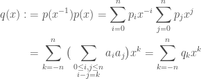
We’ll perform some abuse of notation and use $p$ to also denote the polynomial $p(x):=p_0+p_1x+...+p_nx^n$ . Putting the definition of $\hat{p}(f)$ into the definition of power we have:

$\begin{aligned} power_{f_1, f_2}(p)&=2\int_{f_1}^{f_2}|p(e^{-2\pi\iota f})|^2df \\ &=2\int_{f_1}^{f_2}p(e^{-2\pi\iota f})\overline{p(e^{-2\pi\iota f})}df \\ &=2\int_{f_1}^{f_2}p(e^{-2\pi\iota f})p(e^{2\pi\iota f})df \end{aligned}$

where we have used that, since $p_i$ are real, $\overline{p(x)}=p(\overline{x})$ . We continue by setting:

$\begin{aligned} q(x):&=p(x^{-1})p(x)=\sum_{i=0}^{n} p_ix^{-i} \sum_{j=0}^{n} p_jx^j \\ &=\sum_{k=-n}^{n}\big(\sum_{\substack{0\le i,j\le n\\ i-j=k}}a_ia_j \big)x^k=\sum_{k=-n}^{n}q_kx^k \end{aligned}$

so that

$\begin{aligned} power_{f1,f2}(p) &=2\int_{f_1}^{f_2}q(e^{2\pi\iota f})df \\ &= 2\int_{f_1}^{f_2}\sum_{k=-n}^{n}q_ke^{2\pi\iota k f}df \\ &= 2\sum_{k=-n}^{n}q_k\int_{f_1}^{f_2}e^{2\pi\iota k f}df \\ &= 2\sum_{k=-n}^{n}q_k \frac{e^{2\pi\iota k f}}{2\pi\iota k}\biggr|_{f_1}^{f_2} \\ &= 2\sum_{k=-n}^{n}q_k \frac{e^{2\pi\iota k f_2} - e^{2\pi\iota k f_1}}{2\pi\iota k}. \end{aligned}$

With more abuse of notation, set $q=(q_{-n}, ..., q_n)$ . Also, set

$v_{f_1, f_2}^n := (2\frac{e^{2\pi\iota k f_2} - e^{2\pi\iota k f_1}}{2\pi\iota k})_{k=-n}^n.$

So we have:

$power_{f_1, f_2}(p)=(q, v_{f_1, f_2}^n)$

where $(\cdot, \cdot)$ is the usual dot product. Note that the coefficients of $q(x)$ are also the coefficients of $p(x)\cdot x^np(x^{-1})$ , which is a multiplication of two degree $n$ polynomials and hence can be computed using two FFTs. This shows that the power of a polynomial in a given band can be computed using two FFTs of size $2n+1$ (number of coefficients of $q$ ), some exponentiating, and a dot product. Even though we took our sample rate to infinity, the computation turned out pretty simple.

One more improvement before you go: instead of computing the coefficients of $q(x)$ , we can use the identity

$(q, v_{f_1, f_2}^n)=(Uq, Uv_{f_1, f_2}^n)$

where $U$ is the unitary discrete Fourier transform operator. Since $q$ is a multiplication of polynomials, so a convolution, $Uq$ can be expressed in terms of $Up$ :

$Uq=U(p(x)*x^np(x^{-1}))=Up\times\overline{Up}$

where the $\times$ means component wise. If we already have $Uv_{f_1, f_2}^n$ computed, this means that computing $power_{f_1, f_2}(p)$ takes only a single FFT of size $2n+1$ . Amazing!